Random Forest
Introduction
Random forest is an ensemble method. Ensemble methods combine the predictions of several base estimators built with a given learning algorithm in order to improve generalizability on unseen dataset (reducing overfitting or high variance and reducing underfitting or high bias),
by increasing the robustness of the ensemble method over a single estimator.
More generally, ensemble models can be applied to any base learner beyond trees, in averaging methods such as bagging methods, model stacking, voting, or in boosting.
Random forest is an averaging algorithm ensemble model, making use of a perturb-and-combine techniques: This means a diverse set of classifiers is created by introducing randomness in the classifier construction. The prediction of the ensemble is given as the averaged prediction of the individual classifiers.
Random Forest classifier
As other classifiers, forest classifiers have to be fitted with two arrays: a sparse or dense array n_samples, n_features) holding the training samples, and an array n_samples,) holding the target values (class labels) for the training samples.
RandomForestClassifier
from sklearn.ensemble import RandomForestClassifier
X = [[0, 0], [1, 1]]
Y = [0, 1]
clf = RandomForestClassifier(n_estimators=10)
clf = clf.fit(X, Y)
Randomness in Random Forests
In random forests, each tree in the ensemble is built from a sample drawn with replacement (i.e., a bootstrap sample) from the training set: a subset of observations is used.
Furthermore, when splitting each node during the construction of a tree, the best split is found through an exhaustive search of the feature values of either all input features or a random subset of size max_features, a proces
called feature bagging.
By default, random forest perform both bootstrapped sampling of observations and feature bagging. Boostrap sampling happens once, before the tree construction and feature bagging happens at each split in tree.
max_features parameter: the number of features to consider in a split.
Each tree in the ensemble is built "stochastically" independent* of the other trees in the forest.
In addition, note that in random forests, bootstrap samples are used by default (bootstrap=True).
This means each tree's training set contains the same number of samples as the original dataset, but some samples may be repeated, and others may not be included at all.
On average, a bootstrap sample contains about two-thirds of the original unique samples.
When turned off, the whole dataset (all observations) will be used. So no sampling is applied.
When using bootstrap sampling the generalization error can be estimated on the left out or out-of-bag samples.
This can be enabled by setting oob_score=True.
Random forests are very similar to the procedure of bagging except that they make use of a technique called
- Q: Why is it important to use both bootstrap sampling and feature bagging?
- A: With bootstrap sampling alone, if a feature is very informative, even though all instances in a tree are different, the likelihood of every tree using the most informative feature increases. This in turn would mean that all trees are very similar (correlated), reducing the effectiveness of your ensemble. This requires adding another step "randomness", which is realised by selecting different feature sets to split on at each split in your tree.
Feature bagging works by randomly selecting a subset of the feature dimensions at each split in the growth of individual decision trees. This may sound counterintuitive,
after all it is often desired to include as many features as possible initially in order to gain as much information for the model.
However, it has the purpose of deliberately avoiding (on average) very strong predictive features that lead to similar splits in trees (and thus increase correlation).
That is, if a particular feature is strong in predicting the response value then it will be selected for many trees. Hence, a standard bagging procedure can be quite correlated.
Random forests avoid this by deliberately leaving out these strong features in many of the grown trees.
If all values are chosen in splitting of the trees in a random forest ensemble then this simply corresponds to standard bagging.
A rule-of-thumb for random forests is to use features, suitably rounded, at each split.
The purpose of these two sources of randomness (max_features and n_estimators) is to decrease the variance of the forest estimator.
Indeed, individual decision trees typically exhibit high variance and tend to overfit.
The injected randomness in forests yield decision trees with somewhat decoupled prediction errors.
By taking an average of those predictions, some errors can cancel out. Random forests achieve a reduced variance by combining diverse trees, sometimes at the cost of a slight increase in bias.
In practice the variance reduction is often significant hence yielding an overall better model.
Parameter setting
n_estimators
Refers to the number of trees in the forest. he larger the better, but also the longer it will take to compute. In addition, note that results will stop getting significantly better beyond a critical number of trees.
max_features
Refers to the size of the random subsets of features to consider when splitting a node. The lower the number of features the greater the reduction of variance (the likelihood of overfitting because too complex model with too many features) but also the greater the increase in bias (the likelihood of underfitting because too simplistic model with too little features).
Empirical good default values are max_features=1.0 or equivalently max_features=None (always considering all features instead of a random subset) for regression problems.
Empirical good default values for classification tasks are max_features="sqrt" (using a random subset of size sqrt(n_features), where n_features is the number of features in the data).
The default value of max_features=1.0 is equivalent to bagged trees and more randomness can be achieved by setting smaller values (e.g. 0.3 is a typical default in the literature).
Good results are often achieved when setting max_depth=None in combination with min_samples_split=2 (i.e., when fully developing the trees).
Explainability
feature_importances_
The relative rank (i.e. depth) of a feature used as a decision node in a tree can be used to assess the relative importance of that feature with respect to the predictability of the target variable.
Features used at the top of the tree contribute to the final prediction decision of a larger fraction of the input samples.
The expected fraction of the samples they contribute to can thus be used as an estimate of the relative importance of the features.
In scikit-learn, the fraction of samples a feature contributes to is combined with the decrease in impurity from splitting them to create a normalized estimate of the predictive power of that feature.
By averaging the estimates of predictive ability over several randomized trees one can reduce the variance of such an estimate and use it for feature selection.
This is known as the
The impurity-based feature importances computed on tree-based models suffer from two flaws that can lead to misleading conclusions:
- (1) They are computed on statistics derived from the training dataset and therefore do not necessarily inform us on which features are most important to make good predictions on held-out dataset.
- (2) They favor high cardinality features, that is features with many unique values (such as categorical features with a lot of categories)
Permutation feature importance is an alternative to impurity-based feature importance that does not suffer from these flaws.
In practice those estimates are stored as an attribute named feature_importances_ on the fitted model.
This is an array with shape (n_features,) whose values are positive and sum to 1.0.
The higher the value, the more important is the contribution of the matching feature to the prediction function.
Naive implementation
As discussed, random forest perform both bootstrap sampling of observations and feature bagging.
In this naive implementation, we will only look at bootstrapped sampling to see how four decision trees make up a forest and how a random forest uses
multiple trees with high variance to come to final vote that has less variance.
Decision trees are deterministic, so with the same dataset, each tree should give the same output.
However, when random sampling the observations, the tree can learn a different pattern.
Let's look at a practical example.
| # | feature_1 | feature_2 | label |
|---|---|---|---|
| 1 | 0 | 4 | 1 |
| 2 | 0 | 5 | 1 |
| 3 | 1 | 1 | 1 |
| 4 | 1 | 2 | 1 |
| 5 | 1 | 6 | 0 |
| 6 | 1 | 4 | 1 |
| 7 | 1 | 3 | 1 |
| 8 | 2 | 0 | 1 |
| 9 | 2 | 2 | 1 |
| 10 | 3 | 5 | 0 |
| 11 | 3 | 3 | 0 |
| 12 | 3 | 0 | 1 |
| 13 | 3 | 1 | 1 |
| 14 | 3 | 6 | 0 |
| 15 | 4 | 1 | 1 |
| 16 | 4 | 2 | 0 |
| 17 | 4 | 4 | 0 |
| 18 | 5 | 0 | 1 |
| 19 | 5 | 2 | 0 |
| 20 | 5 | 5 | 0 |
| 21 | 6 | 1 | 0 |
| 22 | 6 | 6 | 0 |
| 23 | 6 | 4 | 0 |
| 24 | 6 | 2 | 0 |
| 25 | 6 | 0 | 0 |
For this example, we'll look at a dataset with 25 instances and two features feature_1 and feature_2
in the context of a binary classification problem.
In the image below we can see our dataset. the X axis shows the value for feature_1 and the Y axis shows the value for feature_2
Each dot in the image below represent an instance its color defines the label: a green label represents the positive class (label=1) and a red label represents the negative class (label=0).
There are 12 positive labelled instances and 13 negative labelled instances in our dataset.
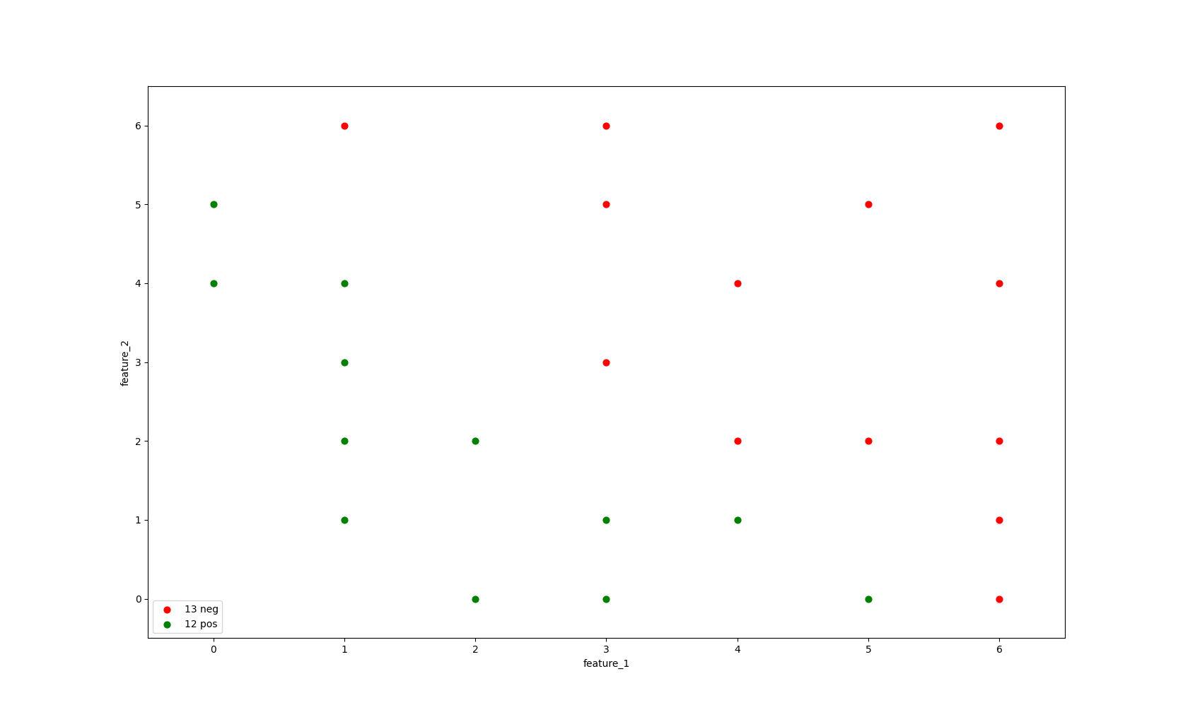
Image 1: Data distribution
If we were to train a decision tree model tree.DecisionTreeClassifier(criterion='entropy', max_depth=1) to find the best split in the data to distinguish between a positive and a negative class, it would create a single split line,
using the information of feature_1 and feature_2 to split the data.
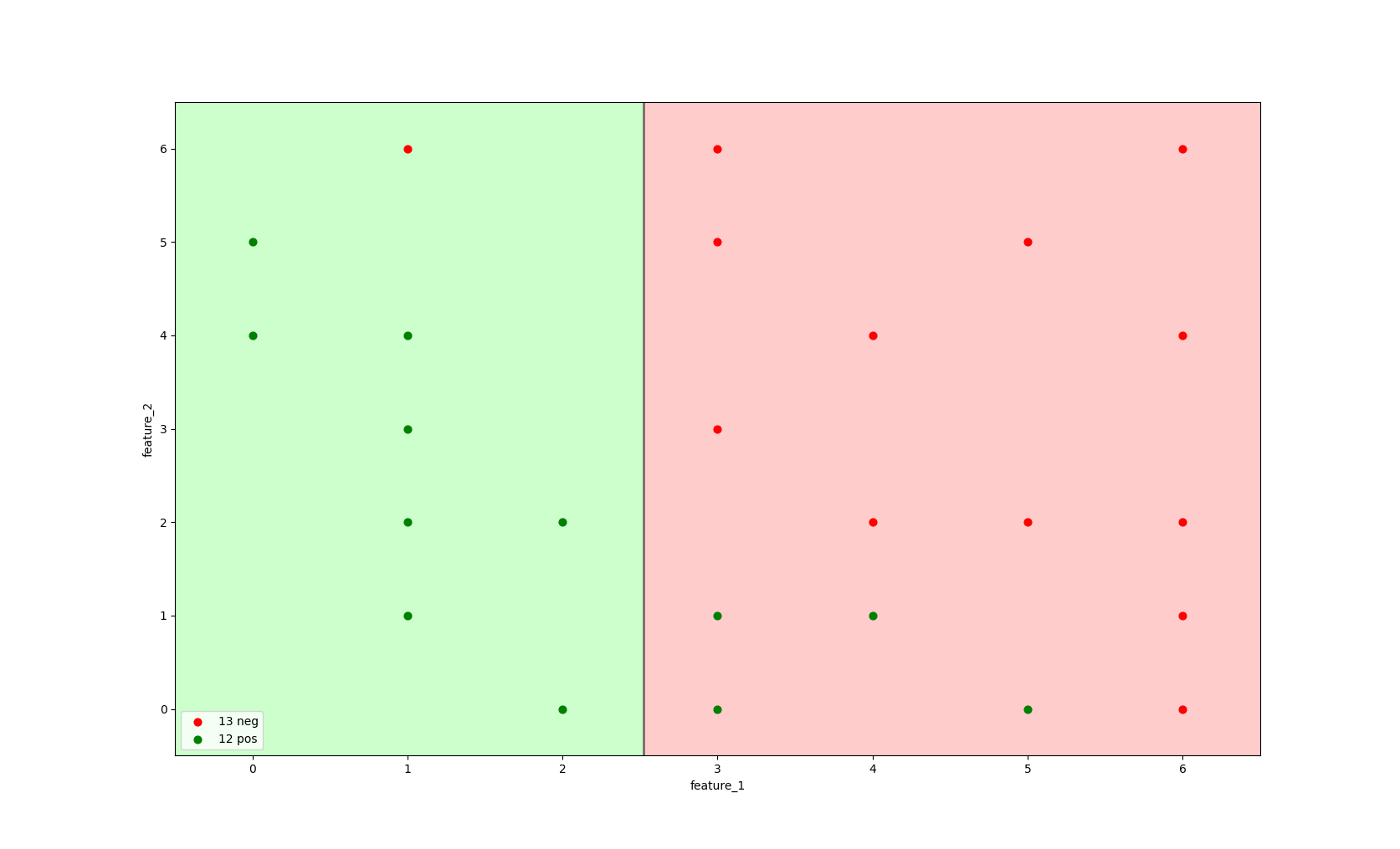
Image 2: Decision tree with max_depth=1 and criterion='entropy' trained on all data.
The image above shows that it would split the data on feature_1 <= 2.5, using the entropy criterion to find the split that gives the most information gain.
The grey line defines the split, everything left of the split is considered a positive class and everything right of
the split is considered a negative class.
Random forests make use of bootstrapped sampling (with replacement) and feature bagging. In this example, we only apply bootstrapping, but not feature bagging.
All decision trees are trained on both feature_1 and feature_2, on a sample drawn with df.sample(fraction=1.0, resample=True).
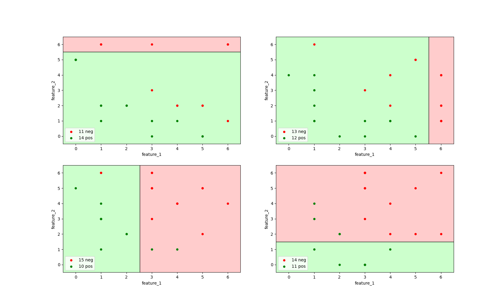
Image 3: Four decision trees with max_depth=1 and criterion='entropy' trained on bootstrapped sample data.
As can be seen from the image above, each of the decision tree on its own does not perform better than the initial decision tree (shown in the bottom-left image).
For instance, the top-left decision tree correctly classifies 3 negative instances as negative (TN), but incorrectly classifies 4 negative instances as positive (FP).
The true power of a random forest becomes visible once we combine our four decision trees in a single classifier. A naive way to visualise this is to increase the max_depth parameter of our decision tree.
A decision tree with more depth can consecutively split on the same two features.
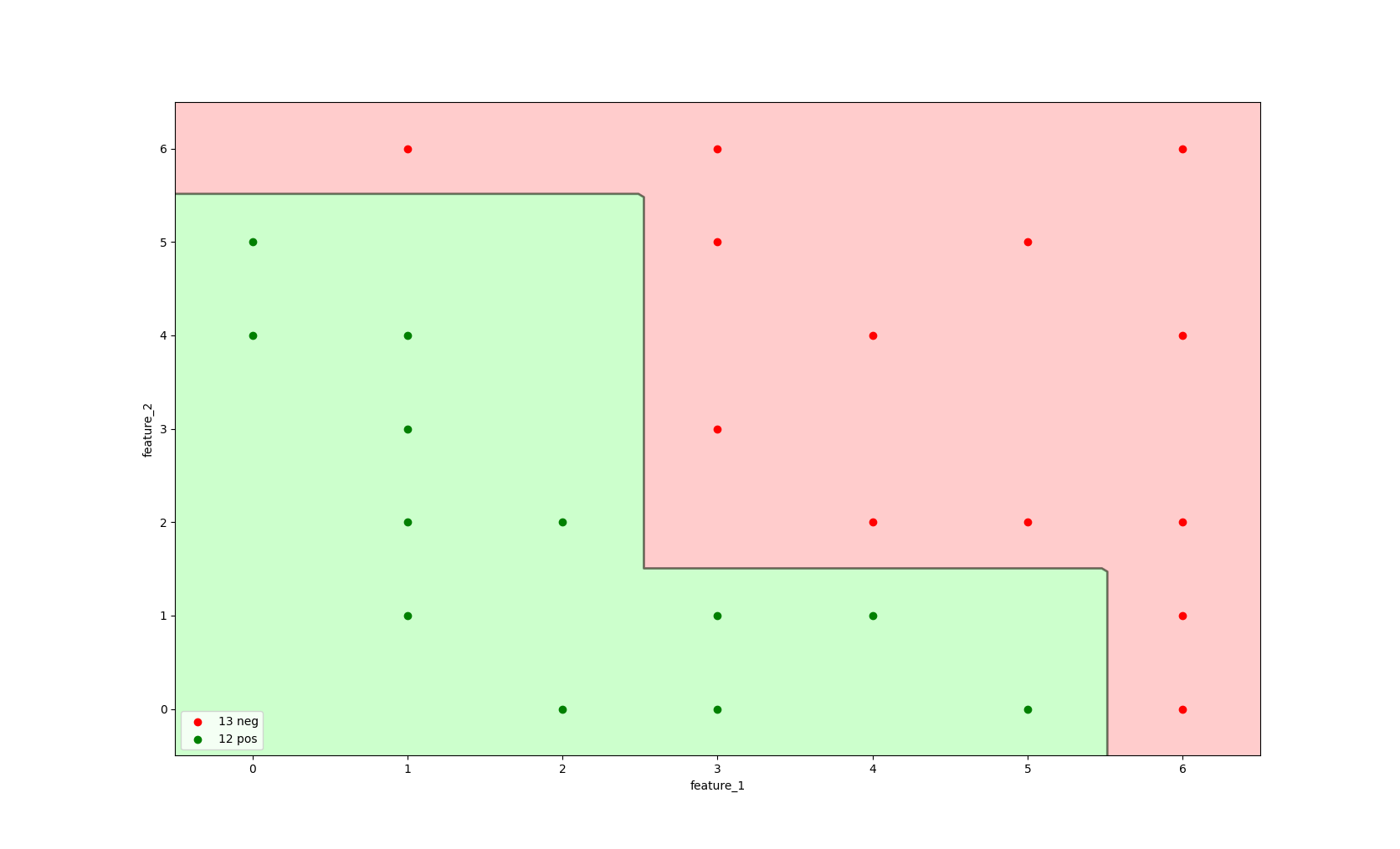
Image 4: A decision tree with max_depth=4, criterion='entropy'.
The image above provides a visual representation of a random forest with four trees, each with max_depth=1, where the final classifier uses the predicted probabilities of each single, high-variance tree.
As can be seen from the image, this random forest model is able to make a more complex split, making use of the information of all underlying decision trees.
This classifier is able to correctly identify negative labelled instances as negative and all positive labelled instances as positive.
In the implementation section we will be able to see that this visual representation is the same as that of the random forest implementation.
- Q: Why not use a Decision Tree with more depth instead of a Random Forest?
-
A: Controlling the depth of a decision tree is difficult. Too shallow of a tree may lead to high bias (underfitting) and a tree that is too deep leads to high variance (overfitting).
Optimal depth analysis is based on heuristics or cross-validation to find the best performing depth that balances bias and variance.
Decision trees with larger depth are very likely to overfit. Random forests are less likely to overfit.
Random forest are more complex as a whole, but each individual tree is less complex than a very deep, single tree. The ensemble approach creates a more robust model.
Implementing a RandomForestClassifier
RandomForestClassifier.fit()
# max_features='sqrt' is the default for ensemble.RandomForestClassifier
# line 337 in tree.DecisionTreeClassifier shows how max_features='sqrt' works
n_features_in_ = 2 # feature_1, feature_2
print(max(1, int(np.sqrt(n_features_in_))))
1

# since we want both feature_1 and feature_2, we choose max_features=2
from sklearn import ensemble
rf_estimator = ensemble.RandomForestClassifier(n_estimators=4, criterion='entropy', max_features=2, bootstrap=True)
rf_estimator.fit(X=df[['feature_1', 'feature_2']].values, y=df[['label']].values)
If we fit the

Image 5: A RandomForestClassifier with n_estimators=100, criterion='entropy', max_features=2, bootstrap=True.
Missing values
A Random Forest estimator has native support for missing values (
Warm start
When set to n_estimators parameter to add to the forest.
Final prediction
- Q: How does a random forest aggregate to get the final prediction?
- A: The predicted class of an input sample is a vote by the trees in the forest, weighted by their probability estimates. That is, the predicted class is the one with highest mean probability estimate across the trees.
In a random forest classifier, the final prediction for an input sample is determined by aggregating the individual predictions of all the trees in the forest.
Each tree votes for a class, and the predicted class is the one that receives the highest average probability estimate across all trees.
This means the final prediction is not just based on the majority vote of the trees, but also considers the confidence (or probability) associated with each tree's prediction.
In other words, random forests aggregate over the
The
This averaging strategy reduces variance and helps to prevent overfitting. By combining multiple individual predictions, which may have their own errors, the ensemble's collective decision-making process leads to a more stable, accurate, and generalizable result.
RandomForestClassifier.predict() & RandomForestClassifier.predict_proba()
predicted_probabilities = rf_estimator.predict_proba(df[['feature_1', 'feature_2']].values)
final_prediction = rf_estimator.predict(df[['feature_1', 'feature_2']].values)
# line 961 in ensemble.RandomForestClassifier shows how the final prediction is made
(np.argmax(predicted_probabilities, axis=1) == final_prediction)
[ True  True  True  True  True  True  True  True  True  True  True  True
  True  True  True  True  True  True  True  True  True  True  True  True
  True]
The following pseudocode explains the process of aggregating the final predictions:
- (1) The final predictions are made by choosing the maximum of the predicted probabilities for each class.
- (2) The predicted probabilities for each class are the averaged predicted probabilities of each tree.DecisionTreeClassifier.predict_proba()
-
(3) The predicted probabilities for each
tree.DecisionTreeClassifierare the sample distribution of the final leaf.
predicted_probabilities and final_prediction
| # | predicted_probability_neg_class | predicted_probability_pos_class | final_prediction |
|---|---|---|---|
| 1 | 0.0 | 1.0 | 1 |
| 2 | 0.0 | 1.0 | 1 |
| 3 | 0.0 | 1.0 | 1 |
| 4 | 0.0 | 1.0 | 1 |
| 5 | 0.75 | 0.25 | 0 |
| 6 | 0.0 | 1.0 | 1 |
| 7 | 0.0 | 1.0 | 1 |
| 8 | 0.0 | 1.0 | 1 |
| 9 | 0.0 | 1.0 | 1 |
| 10 | 1.0 | 0.0 | 0 |
| 11 | 1.0 | 0.0 | 0 |
| 12 | 0.25 | 0.75 | 1 |
| 13 | 0.25 | 0.75 | 1 |
| 14 | 1.0 | 0.0 | 0 |
| 15 | 0.25 | 0.75 | 1 |
| 16 | 1.0 | 0.0 | 0 |
| 17 | 1.0 | 0.0 | 0 |
| 18 | 0.25 | 0.75 | 1 |
| 19 | 1.0 | 0.0 | 0 |
| 20 | 1.0 | 0.0 | 0 |
| 21 | 0.75 | 0.25 | 0 |
| 22 | 1.0 | 0.0 | 0 |
| 23 | 1.0 | 0.0 | 0 |
| 24 | 1.0 | 0.0 | 0 |
| 25 | 1.0 | 0.0 | 0 |
Knowledge cards
Bias & variance
Bias and variance are two types of errors that impact a model's ability to generalize on new data.
Bias refers to the error introduced by approximating a real-world problem with a simplified model, while variance measures how much a model's predictions change when trained on different subsets of the data.
Bias is the difference between the average prediction of our model and the correct value we are trying to predict. High bias indicates that the model is making systematic errors, failing to capture the underlying patterns in the data.
Variance refers to how much the model's predictions change for different training datasets. High variance indicates that the model is sensitive to fluctuations in the training data and may overfit, capturing noise rather than the true underlying relationship.
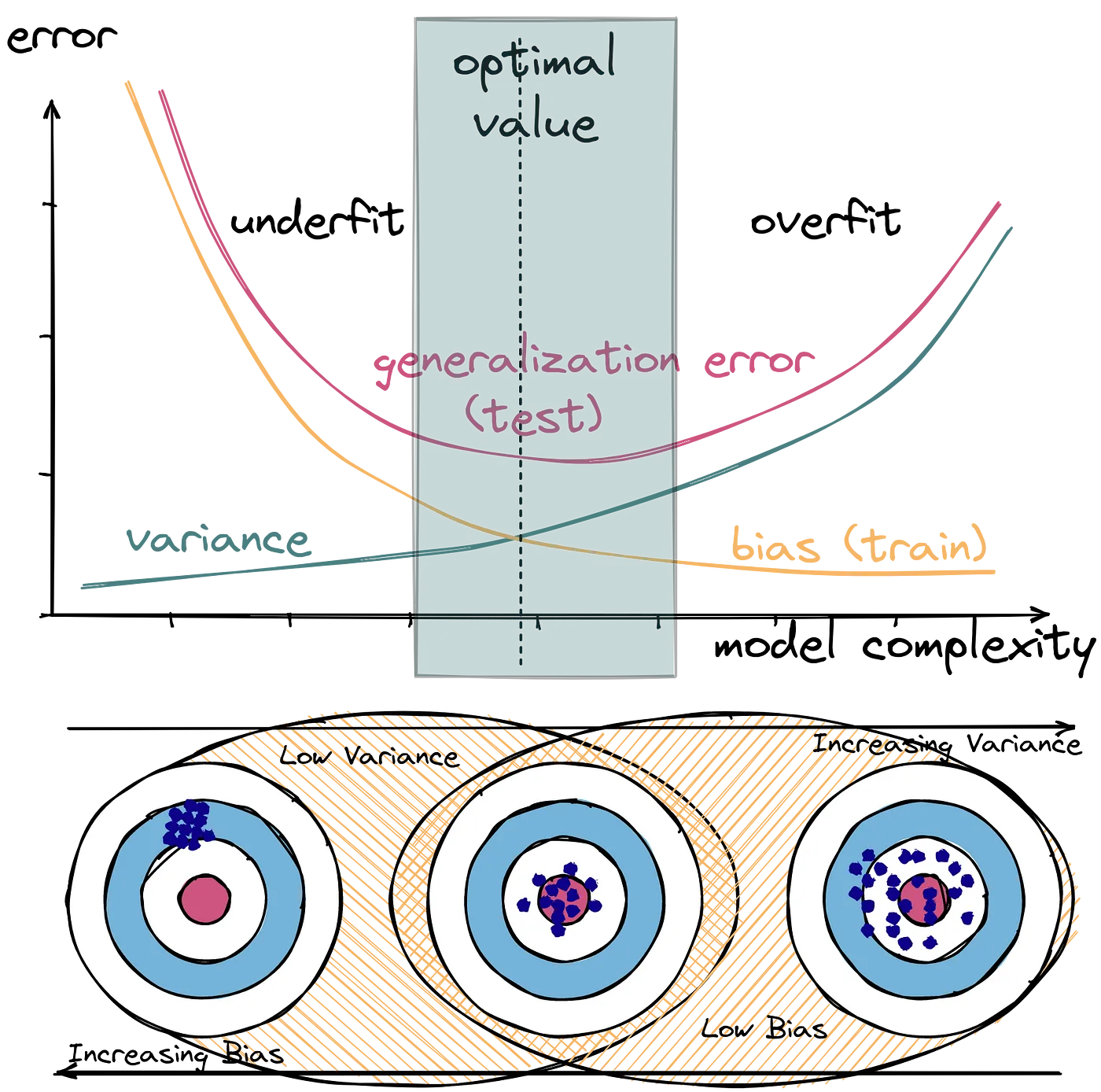
The bias-variance tradeoff highlights the inverse relationship between the two.
High- or low-variance estimator
A high-variance estimator is very sensitive to changes in data.
In the context of decision trees, this means that the addition of a small number of extra training observations can dramatically alter the prediction performance of a learned tree, despite the training data not changing to any great extent.
This risk can be mitigated by using decision trees within an ensemble.
This is in contrast to a low-variance estimator such as linear regression,
which is not hugely sensitive to the addition of extra points–at least those that are relatively close to the remaining points.
Bootstrapping & bagging
Bootstrapping is a statistical resampling technique that involves random sampling of a dataset with replacement.
It is often used as a means of quantifying the uncertainty associated with a machine learning model.
Bootstrap aggregation or bagging combines multiple estimators (such as DTs), which are all fitted on separate bootstrapped samples and average their predictions in order to reduce the overall variance of these predictions.
Carrying out bagging for DTs is straightforward. Hundreds or thousands of deeply-grown (non-pruned) trees are created across
bootstrapped samples of the training data. They are combined in the manner described above and significantly reduce the variance of the overall estimator.
One of the main benefits of bagging is that it is not possible to overfit the model solely by increasing the number of bootstrap samples.
This is also true for random forests but not the method of boosting.