Decision Tree Learning
Introduction
Decision Tree classifier is a type of nonparametric nonlinear supervised machine learning.
A classification or regression decision tree is used as a predictive model to draw conclusions about a set of observations.
In classification decision trees DecisionTreeClassifier leaves represent class labels and branches represent conjunctions of features that lead to those class labels.
Regression decision trees DecisionTreeRegressor can deal with target variables that take continuous values.
- Simple to understand and interpret. Trees can be visualised. Using SHAPley values, feature contributions can be naively understood.
-
The costs of using trees is logarithmic in the number of data points used to train the tree,
O(log N): when the number of data points doubles, the cost increases by a constant. Logarithmic cost is cheaper than linearO (N) - Requires little data preparation, such as data normalization, blank value removal.
- Able to handle multi-output problems: can predict on two or more categorical labels for each input.
- Uses a white-box model: if a given situation is observable in a model. Txhe explanation for the condition is easily explained by boolean logic. By contrast, a black box model results may be more difficult to interpret.
- Decision tree learners can overfit: create over-complex trees that do not generalize the data well. Mechanisms such as pruning, setting the minimum number of samples required at a leaf node or setting the maximum depth of the tree are necessary to avoid this problem.
- Decision trees can be unstable because of small variations in the data might result in completely different trees being generated. This is known as high-variance estimators. This risk can be mitigated by using decision trees within an ensemble.
- Predictions of decision trees are neither smooth nor continuous, but piecewise constant approximations. Therefore, they are not good at extrapolation, estimating values outside of the boundaries of the data used to train a model, c.q.: moving outside of the area populated by the training dataset in a vector space. For instance, if a model is trained on house sizes from 500 square meters to 2000 square meters, it is difficult the predict the price of a 3000 square meters house.
- The problem of learning an optimal decision tree is known to be NP-complete under several aspects of optimality and even for simple concepts. Consequently, practical decision-tree learning algorithms are based on heuristic algorithms such as the greedy algorithm where locally optimal decisions are made at each node. Such algorithms cannot guarantee to return the globally optimal decision tree, c.q. they introduce randomness. This can be mitigated by training multiple trees in an ensemble learner, where the features and samples are randomly sampled with replacement.
- There are concepts that are hard to learn because decision trees do not express them easily, such as XOR, parity or multiplexer problems.
- Decision tree learners create biased trees if some classes dominate. It is therefore recommended to balance the dataset prior to fitting with the decision tree.
- Decision trees are often uncompetitive with other supervised techniques such as support vector machines or deep neural networks in terms of prediction accuracy. However they can become extremely competitive when used in an ensemble method such as with bootstrap aggregation ("bagging"), Random Forests or boosting.
Decision Tree Classifier
The target feature is called the "classification". Each element of the domain of the classification is called a class.
DecisionTreeClassifier.fit()
from sklearn import tree
X = [[0, 0], [1, 1]]
Y = [0, 1]
clf = tree.DecisionTreeClassifier()
clf = clf.fit(X, Y)
clf.predict([[2., 2.]])
array([1])
Decision Tree Regressor
As in the classification setting, the fit method will take as argument arrays X and y, only that in this case y is expected to have floating point values instead of integer values.
DecisionTreeRegressor()
from sklearn import tree
X = [[0, 0], [2, 2]]
y = [0.5, 2.5]
clf = tree.DecisionTreeRegressor()
clf = clf.fit(X, y)
clf.predict([[1, 1]])
array([0.5])
Stopping criteria
In decision trees, stopping criteria define when the tree building process should be halted, preventing overfitting. These criteria include reaching a maximum depth, having too few samples in a node, or observing minimal improvement in splitting criteria like information gain or Gini impurity and can be achieved through the following parameters:
-
max_depthdefines the maximum distance between the root and any leaf. -
min_samples_splitdefines the minimum number of samples required to split an internal node. -
min_samples_leafdefines the minimum number of samples required to be at a leaf node. -
min_impurity_decreasedefines the minimum decrease of the impurity to be able to split a node.
Missing value support
DecisionTreeClassifier and DecisionTreeRegressor have built-in support for missing values using splitter='best'.
For each potential threshold on the non-missing data, the splitter will evaluate the split with all the missing values going to the left node or the right node.
- By default when predicting, the samples with missing values are classified with the class used in the split found during training.
- If the criterion evaluation is the same for both nodes, then the tie for missing value at predict time is broken by going to the right node.
- If no missing values are seen during training for a given feature, then during prediction missing values are mapped to the child with the most samples.
from sklearn import tree
import numpy as np

X = np.array([0, 1, 3, np.nan]).reshape(-1, 1)
X_test = np.array([np.nan]).reshape(-1, 1)
y = [0, 0, 1, 1]

# the samples with missing value are classified with the class used in the split found during training
tree = tree.DecisionTreeClassifier(criterion='entropy', splitter='best').fit(X, y)
tree.predict(X_test)
[1]

# if the criterion evaluation is the same for both nodes, going to the right node ([1])
X = np.array([np.nan, 3, np.nan, 1]).reshape(-1, 1)
tree.fit(X, y)
tree.predict(X_test)
[1]

# if np.nan not seen during training, map to majority class ([1])
X = np.array([0, 1, 2, 3]).reshape(-1, 1)
y = [0, 1, 1, 1]

tree.fit(X, y)
tree.predict(X_test)
[1]
Information gain
Information gain is the basic criterion to decide whether a feature should be used to split a node or not. The feature with the optimal split i.e., the highest value of information gain at a node of a decision tree is used as the feature for splitting the node.
The first thing to understand in Decision Trees is that they split the predictor space, i.e., the target variable into different sub groups which are relatively more homogenous from the perspective of the target variable.
Decision trees follow a top-down, greedy approach that is known as recursive binary splitting. The recursive binary splitting approach is top-down because it begins at the top of the tree and then it successively splits the predictor space. At each split the predictor space gets divided into 2 and is shown via two new branches pointing downwards. The algorithm is termed is greedy because at each step of the process, the best split is made for that step creating a local optimum, without exploring the long-term consequences of that choice. It does not project forwards and try and pick a split that might be more optimal for the overall tree.
In information theory, the entropy of a random variable is the average level of "information", "surprise", or "uncertainty" inherent to the variable’s possible outcomes. In the context of Decision Trees, entropy is a measure of disorder or impurity in a node Since entropy is a measure of impurity, by decreasing the entropy, we are increasing the purity of the data. Another way of describing this is saying that Entropy measures uncertainty with a variable.
When the entropy of a dataset is high, it means that the data is not pure, and the classes are not evenly distributed. On the other hand, when the entropy is low, it means that the data is pure, and the classes are evenly distributed. While choosing an attribute to split, you should choose the one with lowest entropy after the split. Entropy is the uncertainty, so you want to minimise it. As an example, if the split was perfect (all 0's on one side, and all 1's on the other), then entropy will be 0.
Consider a dataset with
Where
is the probability of class i in the dataset
Where
Or in other words
tennis_df
| # | Outlook | Wind | Play |
|---|---|---|---|
| 1 | sunny | False | No |
| 2 | sunny | True | No |
| 3 | overcast | False | Yes |
| 4 | rainy | False | Yes |
| 5 | rainy | False | Yes |
| 6 | rainy | True | No |
| 7 | overcast | True | Yes |
| 8 | sunny | False | No |
| 9 | sunny | False | Yes |
| 10 | rainy | False | Yes |
| 11 | sunny | True | Yes |
| 12 | overcast | True | Yes |
| 13 | overcast | False | Yes |
| 14 | rainy | True | No |
| 15 | sunny | True | No |
| 16 | overcast | False | Yes |
| 17 | rainy | False | Yes |
| 18 | sunny | True | No |
| 19 | sunny | False | No |
| 20 | rainy | True | No |
| 21 | overcast | True | Yes |
| 22 | rainy | False | Yes |
| 23 | sunny | True | Yes |
| 24 | overcast | False | Yes |
| 25 | sunny | False | Yes |
| 26 | overcast | True | Yes |
| 27 | rainy | False | No |
| 28 | overcast | False | Yes |
Consider an example where we are building a decision tree to predict whether to
# probability of the class "No"
p_No = 10 / 28
0.36

# probability of the class "Yes"
p_Yes = 18 / 28
0.64

# calculate entropy
import math
entropy = -(p_No * math.log2(p_No) - p_Yes * math.log2(p_Yes))
print(round(entropy, 2))
0.94

# calculate entropy using scipy
from scipy.stats import entropy
entropy = entropy([p_Yes, p_No], base=2)  # base=2, because in the formula notation we use logarithmic base 2
print(round(entropy, 2))
0.94
There are two features, namely
Wind feature entropy
Splitting the parent node on the attribute
tennis_df[tennis_df['Wind'] == True]
| # | Wind | Play |
|---|---|---|
| 1 | True | No |
| 2 | True | No |
| 3 | True | Yes |
| 4 | True | Yes |
| 5 | True | Yes |
| 6 | True | No |
| 7 | True | No |
| 8 | True | No |
| 9 | True | No |
| 10 | True | Yes |
| 11 | True | Yes |
| 12 | True | Yes |
tennis_df[tennis_df['Wind'] == False]
| # | Wind | Play |
|---|---|---|
| 1 | False | No |
| 2 | False | Yes |
| 3 | False | Yes |
| 4 | False | Yes |
| 5 | False | No |
| 6 | False | Yes |
| 7 | False | Yes |
| 8 | False | Yes |
| 9 | False | Yes |
| 10 | False | Yes |
| 11 | False | No |
| 12 | False | Yes |
| 13 | False | Yes |
| 14 | False | Yes |
| 15 | False | No |
| 16 | False | Yes |
p(No | Wind = True) = 6 / 12
0.5
p(Yes | Wind = True) = 6 / 12
0.5
p(No | Wind = False) = 4 / 16
0.25
p(Yes | Wind = False) = 12 / 16
0.75
Entropy(Wind = True) = -(0.5 * math.log2(0.5)) - (0.5 * math.log2(0.5))
1.0
Entropy(Wind = False) = -(0.25 * math.log2(0.25)) - (0.75 * math.log2(0.75))
0.81
Now let’s see how much uncertainty the tree can reduce by splitting on
Entropy(Parent) = 0.94
Entropy(Wind = True) = 1.0
Entropy(Wind = False) = 0.81

# calculate the weighted average of Entropy for the Wind node
Entropy(Wind) = ((16 / 28) * 1.0) + ((12 / 28) * 0.81)
0.92

# calculate the information gain (IG)
IG(Parent, Wind) = Entropy(Parent) - Entropy(Wind)
IG(Parent, Wind) = 0.94 - 0.92
0.02
Now let's do the same for our
Outlook(sunny)
| # | Outlook | Play |
|---|---|---|
| 1 | sunny | No |
| 2 | sunny | No |
| 3 | sunny | No |
| 4 | sunny | Yes |
| 5 | sunny | Yes |
| 6 | sunny | No |
| 7 | sunny | No |
| 8 | sunny | No |
| 9 | sunny | Yes |
| 10 | sunny | Yes |
Outlook(overcast)
| # | Outlook | Play |
|---|---|---|
| 1 | overcast | Yes |
| 2 | overcast | Yes |
| 3 | overcast | Yes |
| 4 | overcast | Yes |
| 5 | overcast | Yes |
| 6 | overcast | Yes |
| 7 | overcast | Yes |
| 8 | overcast | Yes |
| 9 | overcast | Yes |
Outlook(rainy)
| # | Outlook | Play |
|---|---|---|
| 1 | rainy | Yes |
| 2 | rainy | Yes |
| 3 | rainy | No |
| 4 | rainy | Yes |
| 5 | rainy | No |
| 6 | rainy | Yes |
| 7 | rainy | No |
| 8 | rainy | Yes |
| 9 | rainy | No |
p(No | Outlook(sunny) ) = 6 / 10
0.6
p(Yes | Outlook(sunny) ) = 4 / 10
0.4
Entropy(Outlook(sunny)) = -(0.6 * math.log2(0.6)) - (0.4 * math.log2(0.4))
0.97

p(No | Outlook(overcast) ) = 0 / 9
0.0
p(Yes | Outlook(overcast) ) = 9 / 9
1.0
Entropy(Outlook(overcast)) = -(0 * math.log2(0)) - (1.0 * math.log2(1.0))  # produces a Math domain error, but should return zero.
0.0

p(No | Outlook(rainy) ) = 4 / 9
0.44
p(Yes | Outlook(rainy) ) = 5 / 9
0.56
Entropy(Outlook(rainy)) = -(0.44 * math.log2(0.44)) - (0.56 * math.log2(0.56))
0.99
Now let's compute our Entropy for the
Entropy(Parent) = 0.94
Entropy(Outlook(sunny)) = 0.97
Entropy(Outlook(overcast)) = 0.0
Entropy(Outlook(rainy)) = 0.99

# calculate the weighted average of Entropy for the Outlook node
Entropy(Outlook) = ((10/28) * 0.97 + (9/28) * 0.0 + (9/28) * 0.99)
0.66

# calculate the information gain (IG)
IG(Parent, Wind) = Entropy(Parent) - Entropy(Wind)
IG(Parent, Wind) = 0.94 - 0.66
0.28
The information gain from feature
As previously discussed, entropy measures the randomness in a variable. As we saw, entropy for the
Implementing a DecisionTreeClassifier
Now that we've intuitively understood how to calculate Entropy and corresponding Information gain, let's look at an actual implementation.
For this, we're working with a DecisionTreeClassifier and the same dataset.
DecisionTreeClassifiers can take categorical features, but we need to do some form of encoding to turn the categories into numerical values.
Since there is no logical order between the outlook categories, one-hot encoding is suitable.
For the label, we are using label encoding to convert the "No", "Yes" values into
one-hot encoded features `X` and label encoded `y`
X = tennis_df[['Outlook', 'Wind']]
y = tennis_df[['Play']]

from sklearn.preprocessing import OneHotEncoder, LabelEncoder
enc = OneHotEncoder(sparse=False)
X = enc.fit_transform(X)

le = LabelEncoder()
y = le.fit_transform(y)
When one-hot encoding, you can see that there are three columns for all categories in the
oh_tennis_df
| # | Outlook_sunny | Outlook_overcast | Outlook_rainy | Wind_False | Wind_True | Play |
|---|---|---|---|---|---|---|
| 1 | 1.0 | 0.0 | 0.0 | 1.0 | 0.0 | 0 |
| 2 | 1.0 | 0.0 | 0.0 | 0.0 | 1.0 | 0 |
| 3 | 0.0 | 1.0 | 0.0 | 1.0 | 0.0 | 1 |
| 4 | 0.0 | 0.0 | 1.0 | 1.0 | 0.0 | 1 |
| 5 | 0.0 | 0.0 | 1.0 | 1.0 | 0.0 | 1 |
| 6 | 0.0 | 0.0 | 1.0 | 0.0 | 1.0 | 0 |
| 7 | 0.0 | 1.0 | 0.0 | 0.0 | 1.0 | 1 |
| 8 | 1.0 | 0.0 | 0.0 | 1.0 | 0.0 | 0 |
| 9 | 1.0 | 0.0 | 0.0 | 1.0 | 0.0 | 1 |
| 10 | 0.0 | 0.0 | 1.0 | 1.0 | 0.0 | 1 |
| 11 | 1.0 | 0.0 | 0.0 | 0.0 | 1.0 | 1 |
| 12 | 0.0 | 1.0 | 0.0 | 0.0 | 1.0 | 1 |
| 13 | 0.0 | 1.0 | 0.0 | 1.0 | 0.0 | 1 |
| 14 | 0.0 | 0.0 | 1.0 | 0.0 | 1.0 | 0 |
| 15 | 1.0 | 0.0 | 0.0 | 0.0 | 1.0 | 0 |
| 16 | 0.0 | 1.0 | 0.0 | 1.0 | 0.0 | 1 |
| 17 | 0.0 | 0.0 | 1.0 | 1.0 | 0.0 | 1 |
| 18 | 1.0 | 0.0 | 0.0 | 0.0 | 1.0 | 0 |
| 19 | 1.0 | 0.0 | 0.0 | 1.0 | 0.0 | 0 |
| 20 | 0.0 | 0.0 | 1.0 | 0.0 | 1.0 | 0 |
| 21 | 0.0 | 1.0 | 0.0 | 0.0 | 1.0 | 1 |
| 22 | 0.0 | 0.0 | 1.0 | 1.0 | 0.0 | 1 |
| 23 | 1.0 | 0.0 | 0.0 | 0.0 | 1.0 | 1 |
| 24 | 0.0 | 1.0 | 0.0 | 1.0 | 0.0 | 1 |
| 25 | 1.0 | 0.0 | 0.0 | 1.0 | 0.0 | 1 |
| 26 | 0.0 | 1.0 | 0.0 | 0.0 | 1.0 | 1 |
| 27 | 0.0 | 0.0 | 1.0 | 1.0 | 0.0 | 0 |
| 28 | 0.0 | 1.0 | 0.0 | 1.0 | 0.0 | 1 |
Let's use this information to compute the Entropy of the
oh_tennis_df[oh_tennis_df['x0_overcast'] > 0.5]]
| # | Outlook_overcast | Play |
|---|---|---|
| 1 | 1.0 | 1 |
| 2 | 1.0 | 1 |
| 3 | 1.0 | 1 |
| 4 | 1.0 | 1 |
| 5 | 1.0 | 1 |
| 6 | 1.0 | 1 |
| 7 | 1.0 | 1 |
| 8 | 1.0 | 1 |
| 9 | 1.0 | 1 |
oh_tennis_df[oh_tennis_df['x0_overcast'] <= 0.5]]
| # | Outlook_overcast | Play |
|---|---|---|
| 1 | 0.0 | 0 |
| 2 | 0.0 | 0 |
| 3 | 0.0 | 1 |
| 4 | 0.0 | 1 |
| 5 | 0.0 | 0 |
| 6 | 0.0 | 0 |
| 7 | 0.0 | 1 |
| 8 | 0.0 | 1 |
| 9 | 0.0 | 1 |
| 10 | 0.0 | 0 |
| 11 | 0.0 | 0 |
| 12 | 0.0 | 1 |
| 13 | 0.0 | 0 |
| 14 | 0.0 | 0 |
| 15 | 0.0 | 0 |
| 16 | 0.0 | 1 |
| 17 | 0.0 | 1 |
| 18 | 0.0 | 1 |
| 19 | 0.0 | 0 |
Entropy(Parent) = 0.94

p(No | Outlook_overcast ) =  0 / 9
p(Yes | Outlook_overcast ) = 9 / 9
p(No | Outlook_not_overcast ) = 10 / 19
p(Yes | Outlook_not_overcast ) = 9 / 19

Entropy(Outlook_overcast) = entropy([(0/9), (9/9)], base=2)
0.0

Entropy(Outlook_not_overcast) = entropy([(10/19), (9/19)], base=2)
0.998

# calculate the weighted average of Entropy for the Outlook_overcast node
Entropy(Outlook_overcast) = ((9/28) * 0.0) + ((19/28) * 0.998)
0.677

# calculate the information gain (IG)
IG(Parent, Outlook_overcast) = Entropy(Parent) - Entropy(Outlook_overcast)
IG(Parent, Outlook_overcast) = 0.94 - 0.667
0.272
Let's use
DecisionTreeClassifier
from sklearn import tree
# build decision tree
clf = tree.DecisionTreeClassifier(criterion='entropy', max_depth=3, min_samples_leaf=2)
# max_depth: represents the maximum depth allowed in the tree
# min_samples_leaf: minimum samples required in each leaf node

# fit the tree to tennis dataset
clf.fit(X, y)

feature_names = enc.get_feature_names_out()
target_names = ['Yes', 'No']

# plot decision tree
fig, ax = plt.subplots(figsize=(20, 20))
# tree.plot_tree(clf, filled=True)
tree.plot_tree(clf, ax=ax, feature_names=feature_names, class_names=target_names, filled=True)
plt.savefig('tennis_tree_w_labels.png')
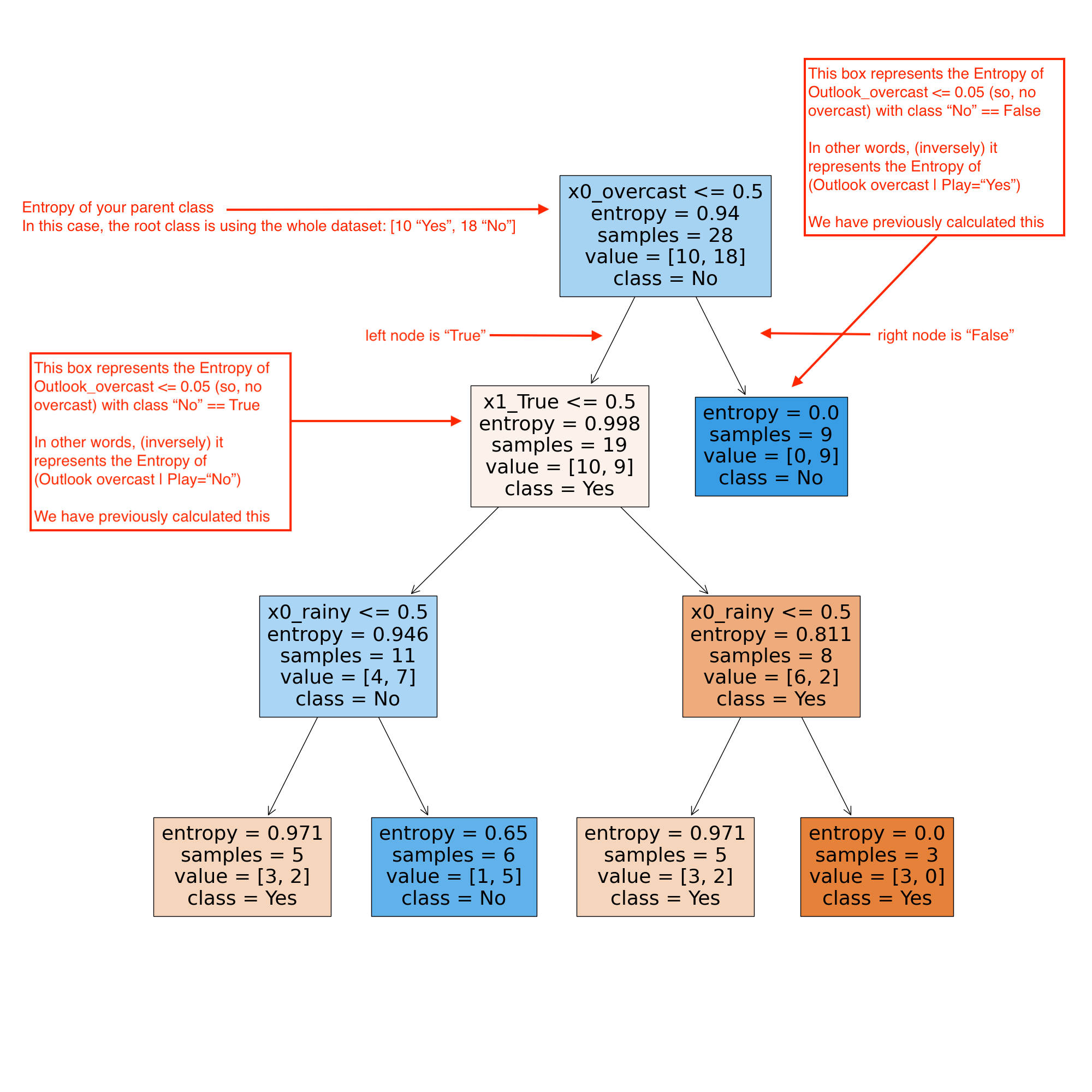
As is shown in the image
Let's have a look at how the decision tree comes to a final prediction.
As we can see in the image above, the features
DecisionTreeClassifier.predict()
# np.array(['Outlook_overcast' 'Outlook_rainy' 'Outlook_sunny' 'Wind_False', 'Wind_True'])
neg_instance = np.array([[0., 1., np.nan, np.nan, 0.],])
clf.predict(neg_instance)
[0]
pos_instance = np.array([[0., 0., np.nan, np.nan, 1.],])
clf.predict(pos_instance)
[1]
If we traverse down the tree for the negative instance prediction, we see
-
(Outlook_overcast <= 0.5); (0 <= 0.5) == True -
(Wind_True <= 0.5); (0 <= 0.5) == True -
(Outlook_rainy <= 0.5); (1 <= 0.5) == False
Our final prediction is class
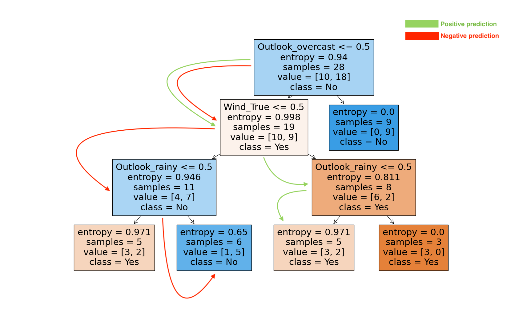
And if we follow the tree for the positive instance prediction:
-
(Outlook_overcast <= 0.5); (0 <= 0.5) == True -
(Wind_True <= 0.5); (1 <= 0.5) == False -
(Outlook_rainy <= 0.5); (0 <= 0.5) == True
Our final prediction is
DecisionTreeClassifier.predict_proba()
clf.predict_proba(neg_instance)
[[0.16666667 0.83333333]]
clf.predict_proba(pos_instance)
[[0.6 0.4]]
Decision tree learning algorithms are generally designed to be deterministic: Given the same training data and algorithm parameters, a decision tree learner will produce the same tree structure and splits each time it is run.
-
Q: Given that a decision tree is deterministic, what does the output of
predict_proba()actually represent? - A: The probabilities are the predicted class probability, which is the fraction of samples of the same class in the final leaf.
If we traverse down the tree for the negative prediction, we see a leaf (2nd from the left) with
If we follow the tree for the positive prediction, we see a leaf (3rd from the left) with
Randomness in Decision Trees
Decision Trees are deterministic by design. However there are a couple of scenarios that can introduce randomness
and there is a random_sate parameter that accounts for this.
First, if there is equal information gain at a split, meaning that both the left node and the right node provide equal information for the decision tree to make a split, the tree can split at random. This is elaborated in this stackoverflow answer.
Second, there can be randomness introduced in some of the algorithms to determine the information gain.
For instance, when the number of features is limited via the max_features parameter,
a randomized list of features is used at each split, which randomized list is presented at each split can be accounted for in the random_state parameter.
Even if max_features = n_features, randomness can still occur.
For instance, the CART algorithm is deterministic by design and finds a global minimum of the weighted Gini indices, however,
a random order in the list of features can mean a split on different features, while still achieving the same Gini index on that split.
Setting the random_state assures that the CART implementation works through the same randomized list of features when looking for the minimum.
As mentioned in the disadvantages section, the problem of learning an optimal decision tree is known to be NP-complete. Practical DT algorithms can therefor rely on heuristics such as greedy algorithms (rather than the more expensive exhaustive search) that produce a local optimum that cannot guarantee a global optimum: what is meant by this is that at each split, the algorithm makes a decision based on an information gain metric, but it does not backtrack at the next split to see if the combined information gain of two splits would have been better if chosen for the previous other option. The algorithm makes a decision and moves on without backtracking that decision at any point.
Explainability
Explainability in machine learning is the process of explaining to a human why and how a machine learning model made a decision.
Model explainability means the algorithm and its decision or output can be understood by a human.
It can be split in global explainability, which refers to human-interpretable insights on the model's overall behavior and
local explainability, referring to insights into why a specific prediction was made for a single instance.
Within the context of a decision tree, since it is a deterministic model, I suppose that the feature_importances_ property represent both global and local explainability.
In a decision tree, the nodes that are split on first are the most important nodes to split on, as they have the largest information gain. The importance of a feature is computed as the (normalized) total reduction of the entropy brought by that feature, also known as the criterion importance.
sklearn._tree.compute_feature_importances()
Feature importance for decision trees are calculated in two steps. [src]
- (1) Calculate importance for each node
- (2) Calculate each feature’s importance using node importance splitting on that feature
(% of samples reaching node
(% of samples reaching left subtree node
(% of samples reaching right subtree node
Using the first node from our decision tree above, the formula is:
= ( 100% x 0.94 — 67.66% x 0.998 — 32.14% x 0.0) / 100
= 0.2647
Where
% of samples reaching node X = 100% = ((10+18) / 28) * 100
% of samples reaching left subtree node X = 67.86% = (19 / 28) * 100
% of samples reaching left subtree node X = 32.14% = (9 / 28) * 100
The second step is to normalize the node's importance by dividing it by all node's importance's: a node’s importance splitting on feature K / Σ all node’s importance.
Complexity
In general, the run time cost to construct a balanced binary tree is
Tree algorithms
ID3 or Iterative Dichotomiser 3 creates a multiway tree, finding for each node (i.e. in a greedy manner) the categorical feature that will yield the largest information gain for categorical targets. Trees are grown to their maximum size and then a pruning step is usually applied to improve the ability of the tree to generalize to unseen data.
C4.5 is the successor to ID3 and removed the restriction that features must be categorical by dynamically defining a discrete attribute (based on numerical variables) that partitions the continuous attribute value into a discrete set of intervals. C4.5 converts the trained trees (i.e. the output of the ID3 algorithm) into sets of if-then rules. The accuracy of each rule is then evaluated to determine the order in which they should be applied. Pruning is done by removing a rule’s precondition if the accuracy of the rule improves without it
CART (Classification and Regression Trees) is very similar to C4.5, but it differs in that it supports numerical target variables (regression) and does not compute rule sets. CART constructs binary trees using the feature and threshold that yield the largest information gain at each node.
Tips on practical use
- Decision trees tend to overfit on data with a large number of features. Getting the right ratio of samples to number of features is important, since a tree with few samples in a high dimensional space is very likely to overfit.
- Consider performing dimensionality reduction (PCA, ICA, feature selection) beforehand to give your tree a better chance of finding features that are discriminative.
- Remember that the number of samples required to populate the tree doubles for each additional level the tree grows to. Use max_depth to control the size of the tree to prevent overfitting.
-
Use
min_samples_splitormin_samples_leafto ensure that multiple samples inform every decision in the tree, by controlling which splits will be considered. A very small number will usually mean the tree will overfit, whereas a large number will prevent the tree from learning the data. Trymin_samples_leaf=5as an initial value. If the sample size varies greatly, a float number can be used as percentage in these two parameters. Whilemin_samples_splitcan create arbitrarily small leaves,min_samples_leafguarantees that each leaf has a minimum size, avoiding low-variance, over-fit leaf nodes in regression problems.
For classification with few classes,min_samples_leaf=1is often the best choice. -
Note that
min_samples_splitconsiders samples directly and independent ofsample_weight, if provided (e.g. a node withm weighted samples is still treated as having exactlym samples). Considermin_weight_fraction_leaformin_impurity_decreaseif accounting for sample weights is required at splits. -
Balance your dataset before training to prevent the tree from being biased toward the classes that are dominant.
Class balancing can be done by sampling an equal number of samples from each class, or preferably by normalizing the sum of the sample weights (
sample_weight) for each class to the same value. Also note that weight-based pre-pruning criteria, such asmin_weight_fraction_leaf, will then be less biased toward dominant classes than criteria that are not aware of the sample weights, likemin_samples_leaf. -
If the samples are weighted, it will be easier to optimize the tree structure using weight-based pre-pruning criterion such as
min_weight_fraction_leaf, which ensures that leaf nodes contain at least a fraction of the overall sum of the sample weights. -
All decision trees use
np.float32 arrays internally. If training data is not in this format, a copy of the dataset will be made. -
If the input matrix
X is very sparse, it is recommended to convert to sparsecsc_matrixbefore calling fit and sparsecsr_matrixbefore calling predict. Training time can be orders of magnitude faster for a sparse matrix input compared to a dense matrix when features have zero values in most of the samples.
Knowledge cards
Parametric vs. nonparametric methods
Parametric methods assume a probability distribution for the given data.
Nonparametric methods do not assume a specific functional form for relationship between the input variables and the target variable.
Nonparametric methods typically require large datasets to make inferences about the underlying distribution.
Linear vs. nonlinear model
The main difference between linear and non-linear models lies in how they represent the relationship between variables.
Linear models assume a straight-line relationship, while non-linear models allow for curves, exponential growth and more complex relationships.
In simpler terms, linear models are easier to understand and analyze, but may not accurately capture real-world data if the relationship isn't truly linear.
Non-linear models offer more flexibility but can be more challenging to interpret and fit to data.
Non-linear models can capture more intricate relationships and patterns in the data, providing a better fit in many cases.
Non-linear models can be more challenging to interpret and require more sophisticated methods for fitting them to data.
An example of a linear model is a linear regression, where the relationship between two variables is modeled with a straight line (y = ax + b).
An example of a nonlinear model is a logistic regression, polynomial regression or a neural network.
Multi-output problem / multi-label / multi-class
Predicts multiple categorical labels. For example, predicting the breed and color of a dog. The model has more than one target variable to predict.
Overfitting vs. underfitting
Overfitting happens when a model generalises too well, learning the noise in the training data
leading to poor performance on new, unseen data. An example is a complex model that perfectly fits a noisy dataset, but performs poorly when presented with slightly different data points.
Overfitting is characterised by high variance, low bias,
good performance on the training data and bad performance on the testing data.
Underfitting, on the other hand, occurs when a model is too simple to capture the underlying patterns in the data,
resulting in poor performance on both the training and test sets. An example is a simple linear model to fit data that has a non-linear relationship.
Underfitting is characterised by low variance, high bias,
poor performance on the training data and bad performance on the testing data.
High- or low-variance estimator
A high-variance estimator is very sensitive to changes in data.
In the context of decision trees, this means that the addition of a small number of extra training observations can dramatically alter the prediction performance of a learned tree, despite the training data not changing to any great extent.
This risk can be mitigated by using decision trees within an ensemble.
This is in contrast to a low-variance estimator such as linear regression,
which is not hugely sensitive to the addition of extra points–at least those that are relatively close to the remaining points.
Bootstrapping & bagging
Bootstrapping is a statistical resampling technique that involves random sampling of a dataset with replacement.
It is often used as a means of quantifying the uncertainty associated with a machine learning model.
Bootstrap aggregation or bagging combines multiple estimators (such as DTs), which are all fitted on separate bootstrapped samples and average their predictions in order to reduce the overall variance of these predictions.
Carrying out bagging for DTs is straightforward. Hundreds or thousands of deeply-grown (non-pruned) trees are created across
bootstrapped samples of the training data. They are combined in the manner described above and significantly reduce the variance of the overall estimator.
One of the main benefits of bagging is that it is not possible to overfit the model solely by increasing the number of bootstrap samples.
This is also true for random forests but not the method of boosting.
Bias & variance
Bias and variance are two types of errors that impact a model's ability to generalize on new data.
Bias refers to the error introduced by approximating a real-world problem with a simplified model, while variance measures how much a model's predictions change when trained on different subsets of the data.
Bias is the difference between the average prediction of our model and the correct value we are trying to predict. High bias indicates that the model is making systematic errors, failing to capture the underlying patterns in the data.
Variance refers to how much the model's predictions change for different training datasets. High variance indicates that the model is sensitive to fluctuations in the training data and may overfit, capturing noise rather than the true underlying relationship.
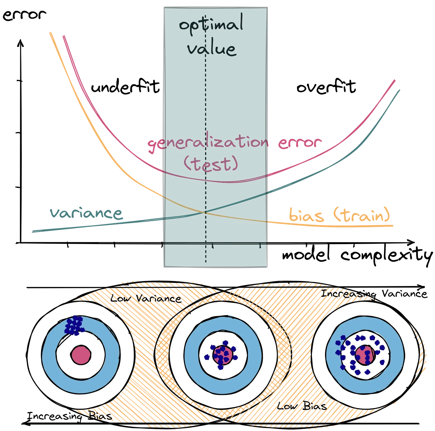
The bias-variance tradeoff highlights the inverse relationship between the two.
Feature encoding
One-hot encoding is a technique used in machine learning to convert categorical data into a numerical format that can be used by algorithms. It represents each category as a binary vector where only one element is "hot" (1) and the rest are "cold" (0). This method is intended for dealing with categorical features that don't have an inherent numerical order (ordinal features). One-hot encoding transforms a categorical column into multiple binary columns, one for each unique category. Can lead to high dimensionality when dealing with many categories, which can be computationally expensive. Using "less than n" approach (omitting one column) can be more efficient. This encoding is needed for feeding categorical data to many scikit-learn estimators, notably linear models and SVMs with the standard kernels.
| # | color | taste |
|---|---|---|
| 1 | green | good |
| 2 | blue | bad |
| 3 | red | bad |
| 4 | red | good |
| 5 | blue | bad |
| 6 | green | good |
| 7 | yellow | bad |
| 8 | red | good |
| 9 | yellow | good |
    import pandas as pd
    from sklearn.preprocessing import OneHotEncoder
    enc = OneHotEncoder(sparse=False)
    X = enc.fit_transform(X)
    X
    [[0. 1. 0. 0.]
     [1. 0. 0. 0.]
     [0. 0. 1. 0.]
     [0. 0. 1. 0.]
     [1. 0. 0. 0.]
     [0. 1. 0. 0.]
     [0. 0. 0. 1.]
     [0. 0. 1. 0.]
     [0. 0. 0. 1.]]
     df = pd.DataFrame(data=X, columns=enc.get_feature_names_out())
| # | color_blue | color_green | color_red | color_yellow |
|---|---|---|---|---|
| 1 | 0.0 | 1.0 | 0.0 | 0.0 |
| 2 | 1.0 | 0.0 | 0.0 | 0.0 |
| 3 | 0.0 | 0.0 | 1.0 | 0.0 |
| 4 | 0.0 | 0.0 | 1.0 | 0.0 |
| 5 | 1.0 | 0.0 | 0.0 | 0.0 |
| 6 | 0.0 | 1.0 | 0.0 | 0.0 |
| 7 | 0.0 | 0.0 | 0.0 | 1.0 |
| 8 | 0.0 | 0.0 | 1.0 | 0.0 |
| 9 | 0.0 | 0.0 | 0.0 | 1.0 |
If we also choose to use one-hot encoding for our label target (y) the taste, we would get two columns LabelEncoder
    from sklearn.preprocessing import LabelEncoder
    le = LabelEncoder()
    y = le.fit_transform(y)
    y
    [1 0 0 1 0 1 0 1 1]
Tree splitting in greedy manner
Greedy splitting in a decision tree refers to the procedure of choosing a single split at each internal node, with the objective of locally optimizing a certain metric (for example, information gain or Gini impurity) without exploring the long-term consequences of that choice.
Essentially, at each node, the split that appears best at that moment is chosen. This method is computationally efficient, but it does not necessarily guarantee a globally optimal solution for the entire tree.
Deterministic vs. probabilistic
Deterministic models produce the exact same output for a given input, following fixed mathematical rules,
while probabilistic models incorporate uncertainty and randomness, providing a probability distribution over possible outcomes instead of a single,
fixed answer.
Deterministic models are predictable and verifiable for applications like regulatory compliance and safety-critical systems.
Probabilistic models are better for environments with noisy data or incomplete information, offering robustness and confidence estimates in areas like medical diagnosis and risk assessment.
NP-complete
@todo;
Global & local explainability
Global explainability refers to human-interpretable insights on the model's overall behavior.
Global explanations offer a holistic view of how the model works, useful for model development and identifying general trends.
An example is a feature importance plot across the whole dataset.
Local explainability refers to insights into why a specific prediction was made for a single instance.
Local explanations are critical for debugging, understanding biases, and ensuring fairness for individual predictions.
An example is specific instance reasoning, such as a human-readable narrative.